What §6.5 actually says
ISO/IEC 17025:2017 §6.5.1 requires that the laboratory establish metrological traceability for its measurements 'through a documented unbroken chain of calibrations, each contributing to the measurement uncertainty'. For pH, the chain usually reads: NIST or NRC primary standard → certified buffer lot → your calibration procedure → your electrode → your sample.
The clause most CALA assessors focus on is §6.5.3: the uncertainty must be documented with sufficient detail to understand what contributes to it. 'Sufficient detail' means a budget that enumerates each contribution, shows how it was estimated, and combines them according to the GUM (Guide to the expression of Uncertainty in Measurement).
This is where the gap lives. Most lab uncertainty statements for pH cover four components: buffer uncertainty, electrode slope drift, temperature compensation, and repeatability. They omit — or implicitly set to zero — the residual liquid junction potential contribution. For many sample matrices, that omitted term is larger than the other four combined.
The real budget, sorted by dominance
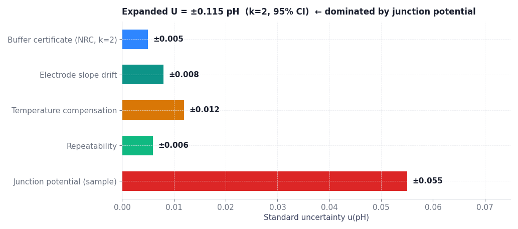
Five components, combined via quadrature per GUM §5.1.2, yield an expanded uncertainty of ±0.115 pH at k=2 (95 % coverage). The individual contributions:
| Component | u(pH) | Source |
|---|---|---|
| Buffer certificate (NRC, k=2) | ±0.005 | CoA from buffer supplier, converted to standard u by dividing by k |
| Electrode slope drift | ±0.008 | Observed variation in slope between calibrations |
| Temperature compensation | ±0.012 | Residual after ATC correction; ±1 °C sample/buffer temperature mismatch |
| Repeatability | ±0.006 | Short-term SD of 10 replicate measurements |
| Junction potential (sample) | ±0.055 | Estimated from matrix type — see Fig. 2 |
Combining: uc = √(0.005² + 0.008² + 0.012² + 0.006² + 0.055²) = 0.058 pH. Expanded U = k × uc = 2 × 0.058 = 0.115 pH. Without the junction potential term, the number would be 0.016 → U = 0.032 pH. The difference is not small. It is 3.5×.
Why the junction potential term changes so dramatically with matrix
The liquid junction is where the calibration buffer (typically 3 M KCl inside the reference) meets the sample. Ideally the two solutions would be identical in ionic composition. They never are. The resulting asymmetric ion diffusion across the junction creates a potential that the Nernst equation does not predict — the residual liquid junction potential (RLJP).
RLJP scales with how different the ionic environment of the sample is from the buffer environment. For pure NIST-style buffers (high KCl, dilute, low ionic strength), RLJP is effectively zero. For real samples, it ranges from small to dominant:
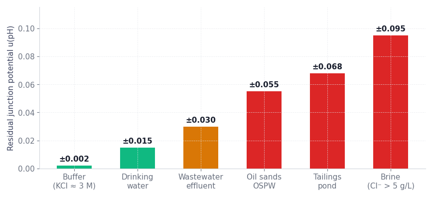
For drinking water and dilute effluent, RLJP is small — the sample is close to the buffer in ionic composition. For oil sands process water (OSPW), tailings pond water, and high-chloride brines, RLJP becomes the dominant uncertainty term by a wide margin.
How to estimate RLJP without specialized equipment
You do not need a Harned cell or a reference-grade Pt-H₂ electrode to estimate RLJP for routine work. Two pragmatic approaches:
Method A — Matrix-matched buffers
Prepare a secondary buffer set in which the background salt matches your sample. Example: for high-chloride brine samples, make secondary buffers in 3 M KCl background rather than nominal ionic strength. Calibrate with the NIST primary buffers, then measure the matrix-matched secondaries. The offset is your RLJP estimate. Publication by Baucke (2002) and Spitzer & Meinrath (2007) document the method; it is accepted for ISO 17025 uncertainty estimation.
Method B — Dilution series
For samples where you cannot prepare matched buffers, measure the sample at full strength and at 1:5 dilution in deionized water. The apparent pH shift minus the true pH shift (from activity coefficient correction) gives an RLJP estimate. Less rigorous than Method A; acceptable for routine matrices with small RLJP contributions.
Writing it up: the certificate language CALA wants
CALA technical assessors have become specific about pH uncertainty language. Avoid 'traceable to NIST via [buffer supplier]'. Instead, write:
That sentence is audit-survivable. It names the chain, the buffer lot, the traceability route, and the dominant uncertainty term — including the matrix dependence that a thorough assessor will ask about.
Summary
- ISO 17025:2017 §6.5 requires a documented uncertainty budget, not just a traceability claim.
- For pH measurements on real matrices, the residual junction potential is the dominant uncertainty term — often larger than buffer, slope, and temperature combined.
- RLJP scales with ionic-composition mismatch: effectively zero for drinking water, ±0.03 for wastewater effluent, ±0.05–0.10 for OSPW, tailings pond, and brines.
- Estimate RLJP with matrix-matched buffers (rigorous) or with a dilution series (pragmatic). Both are defensible for routine work.
- Certificate language should name the SI → NRC → buffer → electrode → sample chain explicitly, and should enumerate the dominant uncertainty contributions — including RLJP.